Snowflake Cost Optimization Essentials for 2024

Snowflake is one of the major cloud data platforms today. Compared to traditional RDBMS, it brings many great features but also new challenges. One of the key advantages is cost effectiveness as Snowflake uses a consumption model for billing the customers. Once the excitement from the new and powerful platform is gone and several use cases are built, teams start thinking how to use the platform effectively and not waste the resources. Additionally given the current economic situation with high interest rates and rising inflation, companies are looking for cost savings. Understanding how Snowflake operates and how to leverage its features effectively can bring significant savings and still provide great performance.

Let’s deep dive into basic optimization techniques which are worth knowing in 2024 whether you are just building your first POC in Snowflake or you are a seasoned pro. We are going to focus on low hanging fruit, things which are applicable at any stage and bring immediate effect. If you are getting into Snowflake world then learning the basics can save you from unintentional cost spikes and angry calls from your budget owners.

‍

1. Snowflake Architecture

Snowflake is Software as a Service (SaaS) which means you do not have to buy any license or hardware. You do not even have to maintain any hardware. All you need to do is sign-up for an account and start using it. Snowflake provides all the HW maintenance for you. Snowflake is cloud agnostic, you can create an account in any of three major cloud providers (AWS, Azure or GCP). Snowflake has 3 layer architecture with Storage, Compute and Cloud Service layer. 

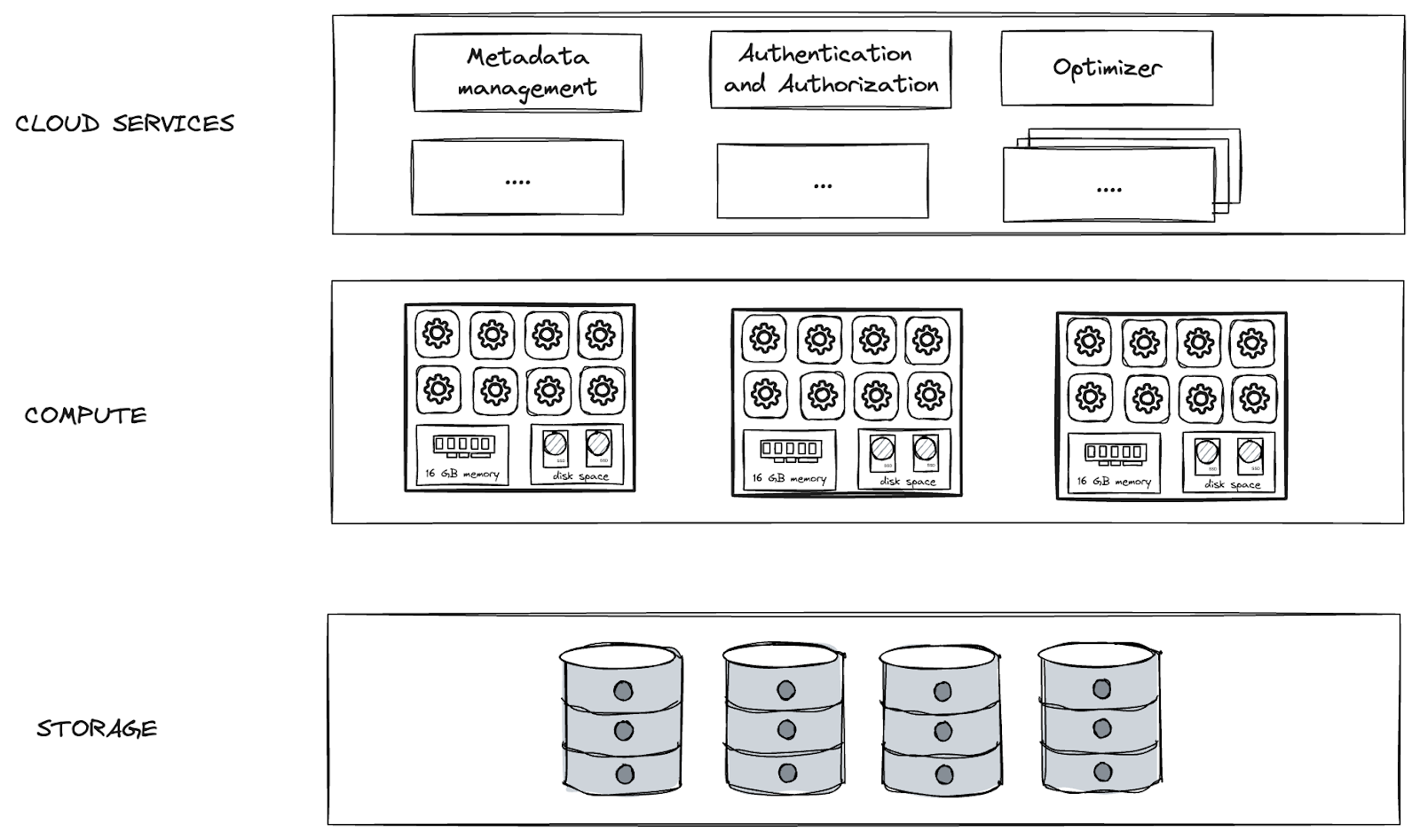
Storage

Storage layer keeps all your data encrypted and compressed. Data are partitioned into immutable micro-partitions which contain between 50 - 500 MB of data before compression. Each table can contain millions of micro-partitions. Apart from live data in your tables, the storage layer also includes data in internal stages, data which are part of Time Travel or Fail-Safe (Continuous data protection).

Compute

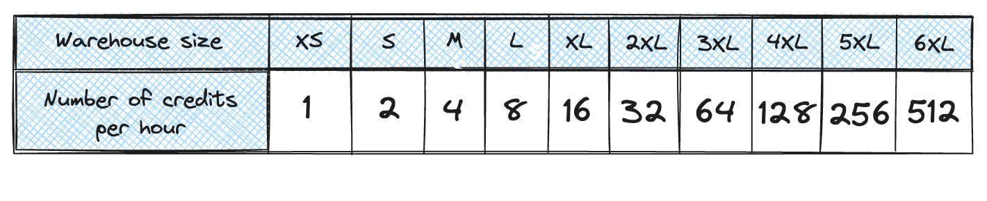
Compute layer does the data processing. It consists of user defined compute clusters, Snowflake calls them Virtual Warehouses. Please do not be confused with the industry term of data warehouse. It doesn’t have anything related to data warehousing and storing data. Snowflake’s warehouse is only compute. Snowflake utilizes T-shirt sizes for warehouse configuration (Extra Small, Small, Medium, etc.). You do not need to specify RAM, CPU power or number of cores. Warehouses differ in the number of nodes. You can take a virtual machine (e.g. EC2) as a node equivalent. Extra Small warehouse has one node, Small has two, Medium four, etc. Each warehouse size doubles the number of nodes. Each node then has 16 GB of memory, 8 threads and local storage for caching purposes. 

Cloud Service Layer

Last architecture layer then takes care about all the background processes of Snowflake execution. Query optimizer, query result cache, metadata management, security & governance, etc. Those are just a few services running inside the cloud service layer.

For more information, check out Snowflake’s official documentation: 

• Key Concepts & Architecture
• Virtual Warehouses Overview

‍

2. Snowflake Billing Concepts

‍Separated Storage and Compute

‍Storage and compute are separated. It means you can easily scale it up or down independently. They are also billed separately with different models. Storage is charged per TB and for compute Snowflake uses usage based pricing. 

‍Usage Based Pricing

‍You are not buying any Snowflake license to use Snowflake Data Cloud. Instead of that Snowflake charges you for processing time = running time of compute clusters. Snowflake uses their own invoiceable unit called Snowflake credit. Price of Snowflake credit is determined by many factors like your Snowflake edition, cloud provider or region. Number of charged Snowflake credits is aligned with the number of nodes in Virtual Warehouse. Extra small warehouse with a single node costs you 1 Snowflake credit for a full hour.Charging is done per second with 1 full minute at the beginning. You will always pay for 60 seconds even though you would suspend the warehouses after 25 seconds. Because Snowflake utilizes usage based pricing your main motivation should be using virtual warehouses (compute clusters) only for necessary time periods and suspend them when they are not needed to prevent wasting of resources and money.

Based on Snowflake architecture you might already suggest that in case of any optimizations we can do it individually for each layer. In the next part of the blog post we are going to share the basic strategies for optimizing your spendings. What you can do to keep your storage cost under control and what you can do to use compute clusters effectively. Let’s focus on low hanging fruit and basic optimization techniques not requiring any deep knowledge.Last but not least, let’s have a look how Snowflake can assist you and what configuration options you should leverage to avoid unnecessary cost spikes.

‍

3. Snowflake’s Cost Management

A good entry point for getting cost distribution understanding is the Cost Management tab under the Admin menu in Snowsight. You can get a general overview about costs for the whole account and easily spot areas which require in-depth analysis. Are you burning so many credits in the last period compared to the previous one? What are the warehouses and queries with the highest cost? Can you see any unexplained spike in storage? You can identify the objects (warehouses, queries, dbs or stages) which require further analysis and break it down. 

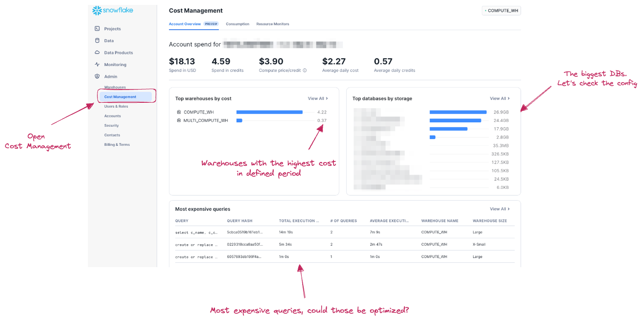
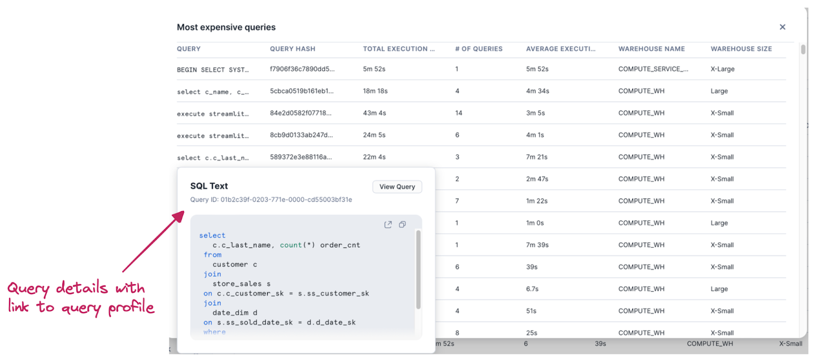
The Cost management tab provides details about most expensive queries with the possibility to easily open the query profile for further analysis. This opens the cost analysis also to users who are not proficient with SQL and writing custom SQL queries to find out that information in metadata would be problematic for them. 

Same applies to storage analysis. For top level overview (on DB level) we can use a chart in the same dashboard. It also provides SQL query which brings data in.

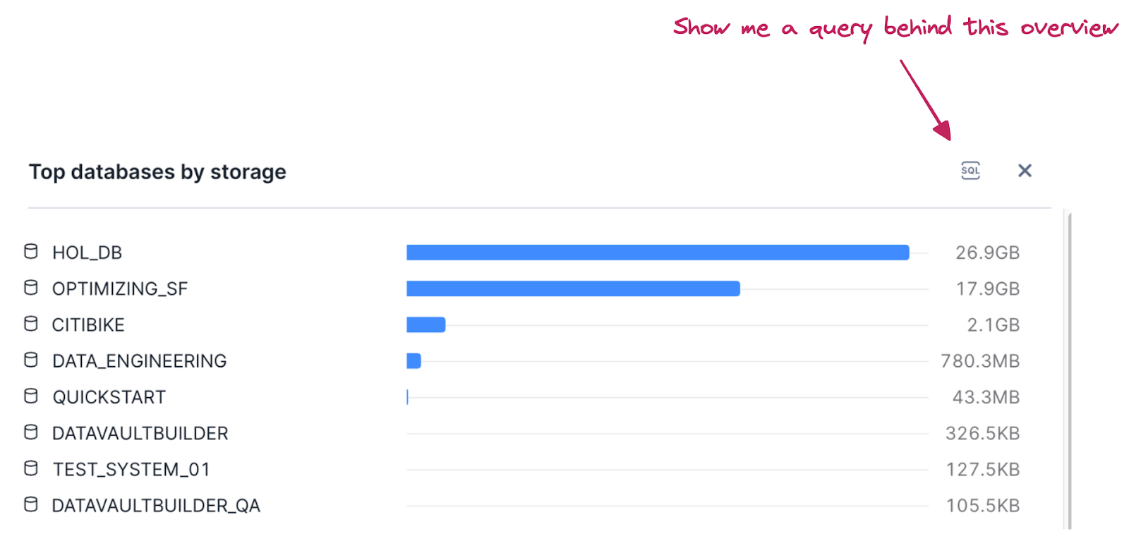
In case we want to go deeper on table level we have to use metadata stored in TABLE_STORAGE_METRICS view in ACCOUNT_USAGE schema inside SNOWFLAKE database.

‍

4. Understanding Snowflake Object Usage

Usage understanding can reveal objects which have been forgotten and maybe could be removed. You can answer questions like:

• Do we have any tables which haven’t been used in the last XYZ days/weeks/months?
• Do we have any data pipelines which refresh data in those unused tables?
• Do we have any dashboards which haven’t been used in the last XYZ days/weeks/months?
• What are downstream dependencies of unused objects?

Keeping unused data in tables you not only might be wasting storage cost, but also impacting compute cost if there are data pipelines to refresh that data on a regular basis. Keeping unused data could also increase risk exposure due to many indirect possible risks like data breach or not being compliant with data privacy regulations. 

Snowflake offers plenty of metadata which can help you to discover such objects. The ACCESS_HISTORY view in SNOWFLAKE database provides an overview of how individual objects are used. Let’s create a popularity analysis to find out unused tables and dashboards. ACCESS_HISTORY provides also data lineage information. From a single place you can check the downstream dependencies before deprecating them. ACCESS_HISTORY view tracks usage on table, view and column level. It provides information about directly and indirectly accessed objects. For example when you query a view, the view columns are directly accessed objects - you can find them direct_objects_accessed column. View is built on top of the same table and this table is indirectly accessed by the view - you can find it in the base_objects_accessed  column. 

Let’s do a simple example to show how you can track data usage by using ACCESS_HISTORY views. We are going to Create a simple table and view on top of it. Then we query the view. After that we will try to find the respective records in ACCESS_HISTORY to understand how it’s tracked and what we can see in different view columns. Please be aware of the latency which is up to 3 hours for the ACCESS_HISTORY. You won’t be able to see the data immediately after running the queries. 

--create a table
create table my_table 
(id number,
name varchar,
value varchar);

--create a view
create or replace view my_view as
select
    id,
    name,
    value
from my_table;

--query a view
select * from my_view;

--query the ACCESS_HISTORY for given query_id
select * 
from snowflake.account_usage.access_history,
where 
    query_id = <your_query_id>;

‍

The DIRECT_OBJECT_ACCESSED column value then contains columns from the view as those ones which have been accessed:

[
  {
    "columns": [
      {
        "columnId": 186374,
        "columnName": "VALUE"
      },
      {
        "columnId": 186373,
        "columnName": "NAME"
      },
      {
        "columnId": 186372,
        "columnName": "ID"
      }
    ],
    "objectDomain": "View",
    "objectId": 163844,
    "objectName": "MY_DB.PUBLIC.MY_VIEW"
  }
]

‍

And BASE_OBJECT_ACCESSED column value contains columns from underlying table:

[
	{
  	"columns": [
    	{
      	"columnId": 184328,
	      "columnName": "NAME"
    	},
    	{
      	"columnId": 184329,
	      "columnName": "VALUE"
  	  },
    	{
      	"columnId": 184327,
      	"columnName": "ID"
	    }
  	],
	  "objectDomain": "Table",
	  "objectId": 161796,
  	"objectName": "MY_DB.MY_TABLE"
	}
]

‍
‍

Based on that information you can easily find all tables which haven’t been queried in the last week or month. Those would be good candidates to investigate them further and find out if you really need them or they can be deprecated. 

You can find more info about ACCESS_HISTORY and how to use it in documentation.

In case you don’t want to build such an observation framework by yourself,Select Star can help you determine what is used and what are the downstream dependencies. Popularity metric shows how often the particular dataset has been queried over a defined time period.
‍

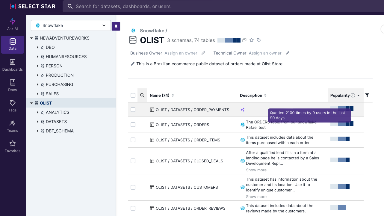
It also has a built-in lineage capabilities that supports many BI tools. This is convenient to check downstream usage directly linked to dashboards.

‍

5. Snowflake Storage Optimization

Now that we’ve identified unused tables and dashboards, let’s continue with a few other storage-related optimizations. 

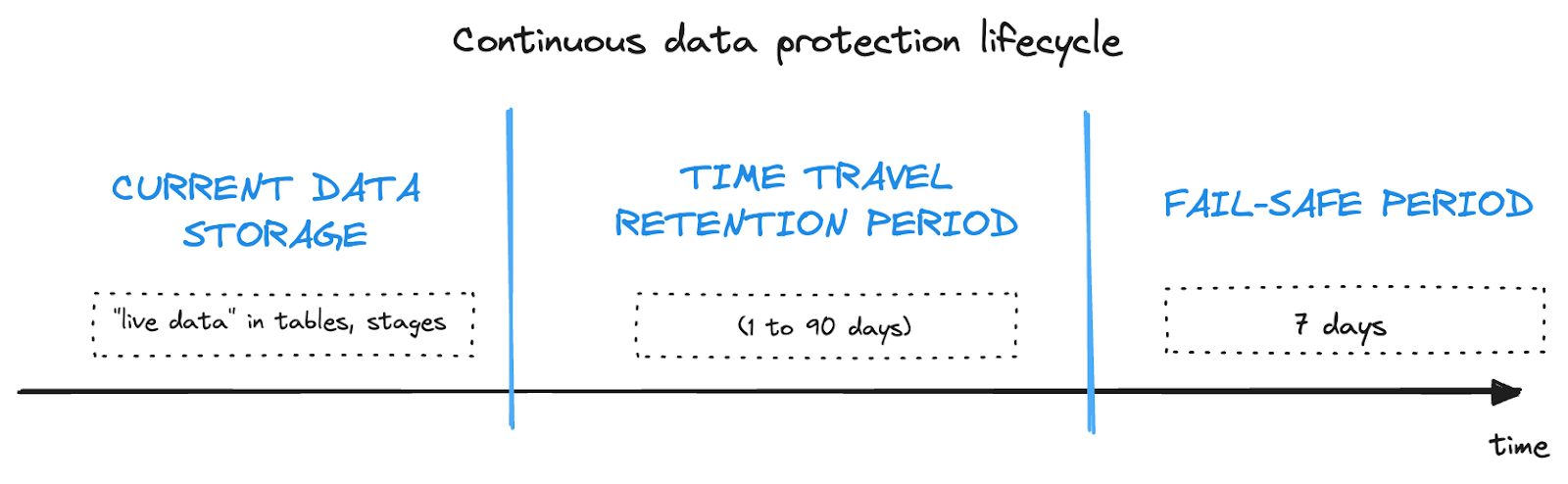
Snowflake Time Travel

Snowflake has a neat feature called Time Travel which keeps old data and allows you to go “back in time“ and bring the old data back in case of failure or errors in the data pipeline. How long back in time you can go depends on settings (1 - 90 days). Standard edition offers only 1 day of Time Travel. Enterprise and higher then supports up to 90 days. Be aware that more days of history means higher storage requirements as Snowflake needs to keep all changes which have been made during the time travel period. 

This feature is enabled by default for all accounts today. My recommendation is to use Time Travel only for business critical data. You do not need it for the stage layer and most probably you do not need it also for all intermediate, working tables.To disable Time Travel, you need to modify the data_retention_time_in_days parameter. You can do it on table, schema, db or account level:

alter schema staging set data_retention_time_in_days=0;

Use Transient Tables 

Snowflake’s transient object type does not have any fail safe period. Fail-safe is a data recovery feature which provides another 7 day period when historical data could be recoverable by Snowflake. Fail-safe starts after Time Travel ends, and it adds another storage cost on top of your regular data storage.

When you define objects (DB, schema, table) as transient, it means you eliminate the fail-safe period and most probably also the time travel period. That could be only 1 day for transient objects.

Given the extra storage and copies Snowflake creates, my recommendation is for all lower environments like DEV, TEST, QA to be built on top of  transient objects.

‍

‍

High Churn Tables

Every update or delete in Snowflake means a new micro partition because they are immutable. If you will be updating the same record multiple times, it can lead to many micro partitions. Especially for large tables, it can cause performance degradation and higher storage cost since the previous data are not deleted but will enter the continuous data protection period, from the time travel and then the Fail-safe features of Snowflake.

You can identify tables with a high frequency of updates, high churn tables, by calculating the ratio of FAILSAFE_BYTES to ACTIVE_BYTES in the TABLE_STORAGE_METRICS view. If that ratio is high you can consider such a table as a high churn table. The easiest solution to solve the higher storage demand for such tables is to use the Transient table type and eliminate Time travel and Fail-safe periods and their storage requirements. 

Data ingestion and file sizing

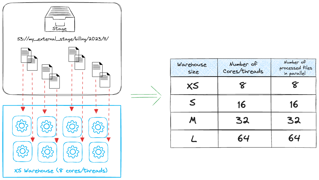
Storage optimization affects also data ingestion phase and particularly how you size your source files. Try to follow the best practices recommended by Snowflake. It says you should be aiming for files between 100 - 250 MB compressed. Try to avoid processing hundreds or thousands of very small files especially when you use Snowpipe because there is an additional overhead fee (0.06 credits per 1000 files). 

Right sizing of the files and number of them also has an impact on warehouse utilization. You need to have a certain amount of files to keep the warehouse busy. The smallest warehouse (XS) has 8 cores and is able to process 8 files (1 per core) in parallel. It is easy to over provision your compute resources for ingestion. Another example, a medium warehouse can process 32 files in parallel. In case you ingest 1 GB of data in 10 files per 100 MB, it’s better to use XS warehouse which will be fully utilized rather than use a Small one when 40% of cores will be sitting unused. 

‍

6. Snowflake Compute Optimization

Warehouse Right Sizing

‍The number one question is always how would I know what is the right size of virtual warehouse for my task? Easy answer is - you need to experiment. Define your SLA for ideal query run time and try different sizes of virtual warehouses. The goal is to find the balance between performance and cost. Would another bigger size bring double speed or significant improvement which is worth the cost? Always start with the smallest available warehouse and increase the size until you find the right size which meets your SLAs. Choose some representative query for testing. This should be a query which processes a typical amount of data.There are also key indicators showing that your virtual warehouse size is lacking in performance which the query needs. The indicator is called spilling.  

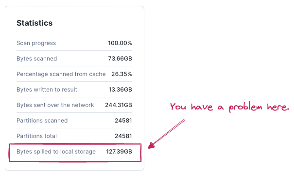
Data Spilling

Spilling indicates the warehouse does not have enough memory to process the data and it offloads the data into local storage. If that is not enough then to remote storage. Remote spilling really kills the performance because it includes network communications which significantly slow down the whole processing. Spilling can be solved by increasing the warehouse size (more memory). This is easiest but could also be the most costly solution. Another way to eliminate spilling is SQL query optimization. That could be complex discipline including different strategies like enabling partition pruning, introducing more filters, optimizing joins, rewriting the query or splitting it into multiple steps. 

Partition Pruning 

Snowflake uses the concept of micro partitions for holding up the data. It’s a storage unit, physical files holding the logical table data. Each table contains thousands of micro partitions. Basic characteristics of micro partitions:

• Max 16 MB of compressed data (50 - 500 MB uncompressed)
• iImmutable - update creates a new micropartition
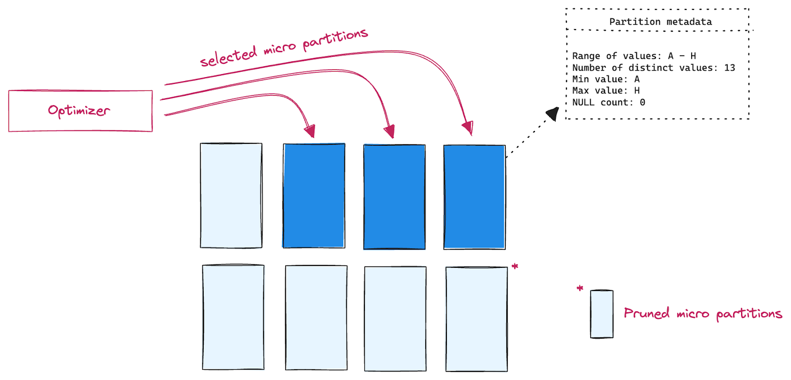
• Snowflake keeps metadata about each micropartition in cloud service layer
• Divides tables horizontally

Because of immutability the micro partitions are a management unit for DML operations. Micro partition metadata is used by the query optimizer to eliminate unneeded micro partitions. Those which contain irrelevant data for a given query.That should always be the number one goal when writing a query. Let’s not read what is not needed, that is the best optimization. How to do that? Data in tables could be clustered according to a defined cluster key or you can leverage natural clustering and storing data along (sorted) columns which are often used in filters or joins. Typically those are timestamp values or different dimensions. It does not make sense to organize data along high cardinality columns like ids. Clustering metadata is then leveraged by a query optimizer to eliminate unneeded micro partitions. 

Scaling

Using the bigger warehouse can solve your pain with performance issues. But do you know when using a bigger warehouse doesn’t make sense? We can either scale the warehouse up or out. Scaling up means resizing the single warehouse (Medium to Large). Scaling out means you add another compute cluster with the same size to make a larger pool of compute resources. Such a warehouse is called a multi cluster warehouse and it can have up to 10 compute clusters. My go-to recommendations for scaling is the following:

• Scale up when you need to boost performance for single query
• Scale up when you need to deal with complex queries on large datasets
• Scale out when you need to solve concurrency issues - peak times with more users, concurrent queries.

Data Refresh

‍Cloud processing has almost infinite options in terms of available compute power. With data lakes on stage the refresh strategy has been „let’s recalculate all data every night“. On the other hand, we have real time data processing bringing new data with minimal latency. Both approaches work but have its price. Evaluate what refresh period you need. Decreasing it might bring significant cost savings. Refreshing data daily not hourly means your virtual warehouse does not need to run almost 24/7. Same goes with incremental processing. If you are able to process only newly coming records, you can significantly lower the amount of processing data and speed up the processing. Many times it does not make sense to move history data back and forth and calculate them every night.  

Snowflake Warehouse Configuration Framework

‍As a final tip let me share the so-called warehouse configuration framework. The way I believe the new warehouses should be created. The sets of parameters which are worth configuring to ensure you are not wasting money. 

• Always enable AUTO_SUSPEND and AUTO_RESUME parameters
• Define the AUTO_SUSPEND according to your workload. Value in minutes for user facing warehouses or warehouses used by downstream apps like reporting tools. For data pipelines use 60 seconds (minimal billing period) and increase when needed. Parameter has impact on local cache availability
• Decrease query timeout parameter from default two days
• Don’t create tens of warehouses but consolidate them
• Don’t let users ability to modify the warehouse configuration - create a few options to use instead
• Assign resource monitors to monitor the cost

Wrapping Up

‍Optimizing performance and cost is a complex discipline requiring deep understanding of the platform, features and possibilities. Snowflake is a great platform to get started on your cloud data warehouse journey, as it can be very flexible depending on your type of workload. There are many ways to turn knobs for its cost and performance. Select Star intelligently tracks Snowflake system metadata and helps govern your Snowflake instance as it grows. Book a demo today to learn more.